Abstract
Because of the real-time requirements, the complexity of the models in a virtual reality application is limited. In our work we applied a preprocessing phase to increase the fidelity of the virtual world while meeting these requirements.
First we focused on the simplification of complex polygon meshes. We found an easy-to-use method to reduce the number of polygons in the model without significant loss in visual accuracy. The polygon reduction algorithm performed so called “edge collapse” operations that removed edges from the model. In our work we compared two simple edge collapsing strategies. During the simplification several variants of different complexity were generated from the same model. During rendering the most suitable variant was chosen using Level of Detail switching technique.
Another focus area of our work was to create realistic light conditions in a virtual world. Although global illumination algorithms generate physically correct light conditions they cannot be applied in a real-time application because of their excessive time consumption. In our work we used textures to map light conditions onto the surfaces. We calculated light conditions in a preprocessing phase using a global illumination algorithm and then we saved the result as textures and we mapped them onto the corresponding surfaces.
Keywords: virtual reality applications, polygon mesh simplification, realistic light conditions, global illumination, textures
1 Introduction
1.1 VR in education
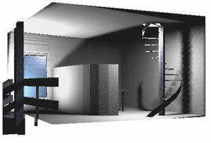
Since there is no health risk when fighting a virtual air battle in a flight simulator or exploring a virtual nuclear power plant in an industrial application (Figure 1), virtual reality (VR) applications became widely used for educational purposes. The aim of these VR applications is to provide employees with a daily routine that is essential for their safety, and to train them how to act in an emergency situation.
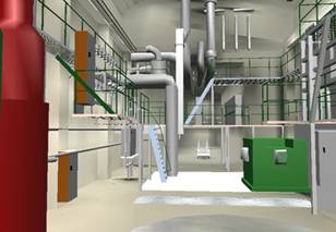
1. Figure – Exploring a nuclear power plant
In a nuclear power plant, because of the radiation exposure, workers may not perform their activities at an arbitrary place and for an arbitrary duration. Using a VR simulator, workers can get acquainted with the complex of the plant without any risk. They can walk through the halls of the plant (as seen on Figure 1), while the radiation level of their environment may be displayed with different colors on the floor. So workers can make an attempt to minimize the radiation dose through avoiding high-radiation areas and following an optimal path during their activity.
1.2 VR requirements
To deceive the user‘s senses in a VR simulator is a rather complex task. A basic requirement is the synchronous operation of the different devices. Any inaccuracy will result in dramatic decrease in realism. For example, if computing time increases because of a realistic, large polygon model, the simulator will only be able to respond to the user interaction with a significant delay. If the user turns his/her head to the side, the view appearing on the display of the VR-helmet will only follow this movement with a delay that maybe cannot be noticed directly, but may result in the fatigue and dizziness of the user. This phenomenon is called the “simulator disease”.
Because of the possibility of the simulator disease effective visualization algorithms are needed that meet both real-time requirements and increasing user demands. Our goal was to increase the fidelity of the virtual models while keeping real-time requirements. The two focus areas we dealt with were mesh simplification techniques and realistic light conditions using textures.
2 Mesh simplification techniques
We were looking for an easy-to-implement method which was able to reduce the number of polygons in the model without significant loss in visual accuracy. Firstly, two existing mesh storage techniques will be described: Level of Detail switching and progressive meshes.
2.1 Mesh storage techniques
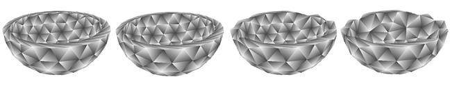
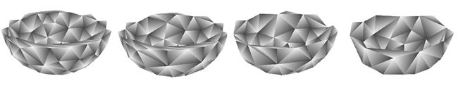
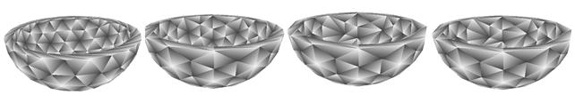
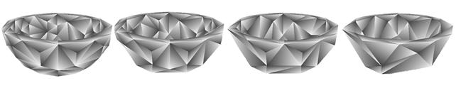
Level of Detail (LOD) switching is the simplest solution to the problem of mesh complexity. In this approach different variants of the same model are created and they are stored independently (see Figure 2). These variants are prepared in an off-line preprocessing phase. Because of the limits in storage capacity only a few (e.g. three) variants can be used. At every moment of the rendering, the most adequate variant is chosen. That means we choose the less complex variant that produces an image quality “good enough”. When zooming in to an object, switching between the different variants may cause rough visual transitions called “popping effect”.
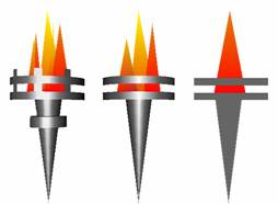
2. Figure – Different LOD variants of a torch
Progressive meshes (PM) represent a more sophisticated storage technique (see [1], [4]). Unlike LOD switching (where the variants are stored independently), a progressive mesh is stored in a form of a coarse base mesh and a sequence of detail records. These records are used to refine the base mesh into the original mesh. During rendering, the most adequate variant of the model is constructed by applying the detail records one after another to the base mesh until the resulting mesh becomes “good enough”.
Although progressive meshes represent an excellent and natural approach to the problem of level of detail, they need some extra data structures and processing time during rendering. On the other hand, LOD switching can easily be implemented even in a single VRML file (VRML supports a node called “LOD”, see [2]). That is why we preferred LOD switching when choosing a storage technique.
2.2 Generating mesh variants
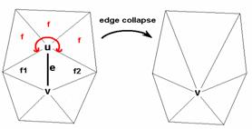
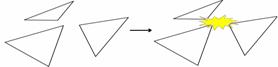
To generate the different mesh variants an operation called edge collapse is used. This operation removes an edge and two adjacent faces from the model (see Figure 3). The edge will be replaced with a single vertex. If we apply the edge collapse operation several times to the original mesh we will get ever coarser meshes.
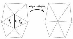
3. Figure – The edge collapse operation removes an edge from the model
In each step a criterion is used to choose the most “adequate” edge to collapse. In our implementation we used a so-called local criterion. Local criteria consider only the actual mesh before performing an edge collapse operation on it. They “forget” the original mesh so there is no guarantee that the resulting base mesh will even be similar to the original one. (Moreover, a continuous mesh will probably break up, as you may see in the appendix.) In return, this algorithm is much faster than the algorithms based on global criteria that “remember” the original mesh.
First we performed the edge collapse operations using the following simple formula (see Formula 1). The meaning of the symbols is as follows: e is the actual edge; f1 and f2 are its neighbor faces.
![]()
1. Formula – a simple local criterion
According to the formula, a longer edge will have a higher cost than a shorter one, because of the bigger nominator. Similarly, larger “crack” along the edge means larger difference in the face normals, resulting in smaller dot products that imply smaller denominator and higher cost. For example, when the angle between the face normals is a right angle, then the denominator becomes zero and the cost becomes infinite (see Fig. 4).
4. Figure – How cost depends on the angle between the two adjacent faces
A problem with Formula 1 is that it is “short-sighted”. It only takes into account those two faces that are adjacent to the edge under examination. The neighbors of these two faces are not considered. In order to show the importance of this issue let us take a cube and one of its diagonals (shown with an arrow on Figure 5)! The normals of the adjacent faces are parallel, so the nominator is 1, which is its largest possible value, so the cost is minimal. That means this operation will be performed as one of the very first edge collapses, although it causes a considerable change in the mesh topology (see the right side of Figure 5).
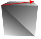
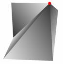
5. Figure – A cube before and after an edge collapse operation
In order to avoid the aforementioned problem and to improve the quality of the result, a more sophisticated formula is needed. An easy-to-use formula was found in the article of Melax ([3]) (see Formula 2):
![]()
2. Formula – a more sophisticated local criterion
The meaning of the symbols is as follows (see Figure 6 for the notation): e is the edge being examined; u and v are its end points. Faces f1 and f2 are the neighbors of the edge e. The set F represents the faces that are adjacent to vertex u, but not adjacent to vertex v. Let us call them “semi-adjacent” to the edge e.
6. Figure - Notation used in Formula 2
As we can see, this formula is asymmetric, since it describes the cost of collapsing vertex u into vertex v. To calculate the opposite direction (collapsing v into u), we have to repeat the calculations with a different F set of faces.
Unlike the previous one, this formula does take care of the neighborhood of the disappearing vertex (u). Namely, from this neighborhood the “most expensive” face is considered.
Let us consider an adjacent face (f1 or f2) and a semi-adjacent face (i.e. from the set f)! The cost they define depends on the angle between their normals as shown on Figure 8.
7. Figure – How cost depends on the angle between an “adjacent” and a “semi-adjacent” face
On a flat surface, for example, the angle between the normals of the aforementioned faces is zero, that means their dot product is 1, resulting in a minimal cost of 0.
On a cube, if we consider one of its diagonals (see Figure 5 again), the angle between the adjacent and semi-adjacent faces is a right angle, resulting in a cost of 0.5. This high cost will delay the collapse of this edge until there are no other edges with a lower cost.
2.3 Implementation
After discussing the principles of mesh simplification techniques, here follows a detailed explanation of our implementation. The application was implemented in Java. It receives a polygon model in an input VRML file, generates different levels of detail using Java3D, and then saves them as VRML output files.
In order to import the initial VRML file into Java3D, we used the class VRML97Loader of the package org.web3d.j3d.loaders. This class loaded the content of the VRML file and transformed it into a Java3D scene graph (about Java3D and scene graphs see [7], [8] and [9]).
During the importation of the VRML file, shapes were automatically tessellated into triangles and rectangles. But face indexes and vertex indexes were lost during the loading, resulting in a set of "independent" faces, and only containing the topological information implicitly.
After loading the model we had to recover this topological information (Figure 8) by separating vertex information and face information from each other. We took polygons one after another and examined their vertices. New vertices were inserted into a vertex list. Vertices found in the vertex list were referenced further on with their indices.
8. Figure – Recovering topological information
After recovering explicit topological information we were ready to perform edge collapse operations. In each step, the edge with minimal cost was eliminated. The resulting mesh is periodically saved into separate files that will be at last composed into a single VRML file using the LOD node. So switching between the different representations is made automatically by the VRML browser.
In order to make edge collapses visible during the simplification process, faces of the model were displayed in a specific way. Three different shades of grey were specified and these colors were bound to the vertices of each triangle in a random order, as seen on the Figure 5. So, in most cases, adjacent faces received different colors along their common edges, making edges easy to observe. In order to ease the examination of the model arbitrary rotation of the model was allowed.
In order to facilitate the simplification of large polygon models, so-called interaction points were introduced. Instead of displaying (and saving) the result after each simplification step, the result was only displayed and saved at the interaction points. The number of simplification steps between two interaction points was defined by the user. For example, if a step of 1000 was given, files containing …, 3000, 2000, 1000 polygons were created.
The application can be used for demonstration purposes, as well. In this case, the program stops at each interaction point, highlights the next edge to be collapsed and waits for a mouse click. In order to reduce the number of clicks when the number of the polygons is large, a threshold can be specified, and a mouse click is only needed at an interaction point if the number of polygons is less than the given threshold.
3 Realistic light conditions using textures
When using a VR application, light conditions are expected to be similar to those in the real physical world. But in a real physical environment light conditions depend not only on the light sources that illuminate the object directly, but on the lights reflected from all other objects, too. Because of this coupling between the objects, the time consumption of the global illumination algorithms (that are able to calculate physically correct light conditions) is extremely high, so there is not enough computing capacity to apply global illumination in VR applications.
One possible solution to the problem is the application of an off-line preprocessing phase. During this phase, light conditions could be calculated and the result could be mapped onto the surfaces in a form of textures. Since these textures are static (they act like wallpaper), they are not suitable for specular materials, such as a mirror. More precisely, since the light conditions that are mapped onto the surfaces do not depend on the viewer’s position, they can only be applied in case of diffuse lightning, e.g. a whitewashed wall. In case of specular lightning, light conditions cannot be “glued” on the surface.
3.1 RenderX – a global illumination software
We applied “RenderX” global illumination software to calculate the light conditions ([5], [6]). The RenderX software opens a VRML file, calculates the light conditions using various methods for global illumination, and saves the resulting light conditions into an XML file in the form of RGB values.
In order to increase image quality, RenderX tessellates large triangles into smaller ones before running the global illumination algorithm. The XML output file will contain RGB information for each small triangle called “patch”.
3.2 Implementation
We developed an application that read the XML file and loaded RGB values of the patches into an internal data structure. The next step was to identify the patches that originate from the same triangle. In order to reduce the amount of computing, all patches lying in the plane of the given triangle were selected. Using a simple coordinate transformation, these patches were transformed to be facing to the camera and they were scaled to fit into the window. In this moment the patches were ready to make a “snapshot” of them. Using Java3D raster operations, a rectangular window of the screen was read and saved into an image file. After computing the coordinates of the vertices in the texture space we could map the texture onto the original mesh.
The RenderX output contains a single RGB value for each patch. When using only one color per patch for drawing, edges between patches become visible. To avoid this, we derived a color value for each vertex. (That means we will be able to draw a patch using three RGB values.) The color of each vertex was composed by using the color of the adjacent patches. Each patch color was weighted with the angle belonging to the patch at the examined vertex.
4 Results
4.1 Mesh simplification
It is an important issue whether the algorithms are able to preserve sharp “cracks” on the surface called discontinuities. In order to test the aforementioned formulas we created an ellipsoidal shape with a cylindrical hole in it (see the left side of Figure 9). When we reduced the shape with first formula, the algorithm was unable to preserve the discontinuity around the hole (see the right side of Figure 9).
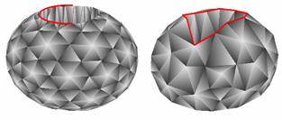
9. Figure – An ellipsoidal shape reduced with the first formula (452 and 200 faces)
Despite its simplicity and locality the second formula produced surprisingly faithful results. It was able to preserve the discontinuities of the model as shown on Figure 10.
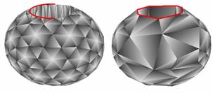
10. Figure – The same shape reduced with the second formula (452 and 200 faces)
The problem with both formulas is that each formula consists of two factors, “length” and “smoothness”. These factors are coequal so they are able to compensate each other. For example an edge representing a sharp discontinuity may have a low cost when the edge is short enough. So a discontinuity on the surface may disappear during the simplification if it consists of short edges.
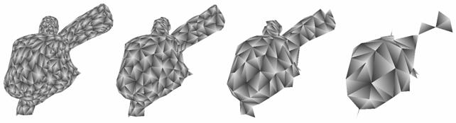
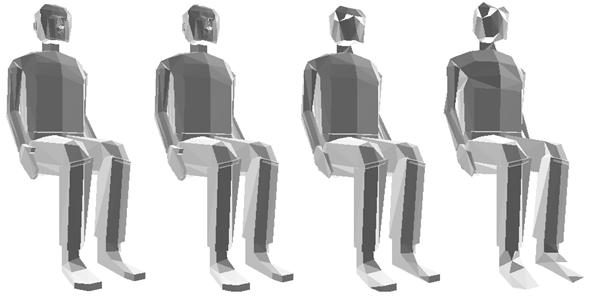
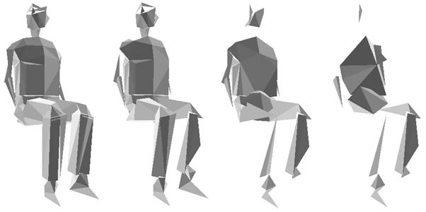
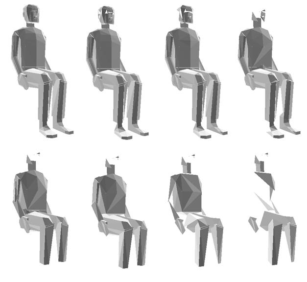
Remark. More examples for mesh simplification can be found in the appendix.
4.2 Lightmaps
In order to demonstrate the results after processing the RenderX output, the following VRML scene was chosen (see Figure 11):
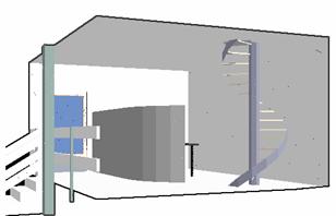
11. Figure – A simple VRML scene displayed by a VRML browser
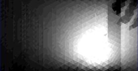
There are two light sources in the VRML world (the VRML browser did not display them). We loaded the model into RenderX and we got a snapshot of the virtual world as shown on Figure 12. Due to the physically correct calculations light sources and shadows became visible.
12. Figure – The output of the global illumination algorithm
Using our application we can extract the light conditions on the wall behind the stairs (Figure 13). Using the aforementioned trick we can produce three RGB values for each triangle (Figure 14).
13. Figure – Texture generated from the RenderX output (wall behind the stairs)

14. Figure – Smooth version of the same texture
Another possible applications of lightmaps:
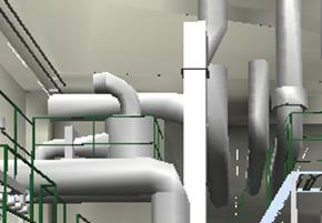
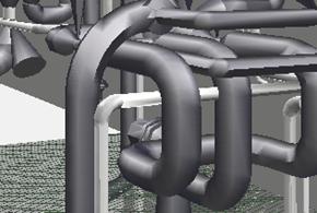
15. Figure – Textured pipes in an industrial application
5 Conclusion and future work
On the previous pages we provided an overview of the methods that can be used in a VR simulator to enhance reality without radical increase of computing work. Both mesh simplification and lightmaps were tested with simple models and produced adequate results.
In the future, a more user-friendly mesh simplification application could be developed and it could be used as a demonstrating tool. It would be nice to make a comparison between different local and global edge collapse strategies.
Interesting light effects could be achieved with the use of more than one texture per face. For example, depending on the viewer’s position, different textures could be used.
Acknowledgements
We would like to say thank you to our supervisor László Szirmay–Kalos for his continuous help and support during the development and for the lots of useful tips given.
References
[1] Hugues Hoppe: Progressive Meshes. In ACM SIGGRAPH 1996, pages 99-108.
[2] A. L. Ames, D. R. Nadeau, J. L. Moreland: VRML 2.0 sourcebook. John Wiley & Sons, Inc. 1997
URL: http://www.melax.com/polychop/gdmag.pdf
[4] M. Grabner: Multiresolution based on View-Dependent Progressive Meshes. CESCG 1999.
URL: http://www.cg.tuwien.ac.at/studentwork/CESCG99/ MGrabner/
[5] Szirmay-Kalos, L.: Monte-Carlo Methods in Global Illumination. Institute of Computer Graphics, Vienna University of Technology, 1999
URL: java.sun.com/products/java-media/3D/collateral/
[8] Java 3D Tutorial, URL: www.java3d.org/tutorial
[9] Java 3D FAQ, URL: www.j3d.org/faq/intro.html
Appendix